Gradient Domain Fusion • steven.codes

This post is a modified version of a site that I submitted for a project in my image manipulation class with Alexei Efros.

On this page, I give some quick explanations of some algorithms, but the main focus is to display and compare results. The base technique is called Poisson Blending. Its goal is to blend a source image into a target image. It accomplishes this by defining constraints based on the gradients of the pixels in the result image. These constraints can be grouped to form a least-squares problem, which can be represented in sparse matrices and solved by a library least-squares solver.

Toy Problem: Reconstruction

To get used to formulating the pixel constraints as least squares problems in sparse matrices, first I practiced simply reconstructing an image given its gradient constraints and a single pixel intensity value.

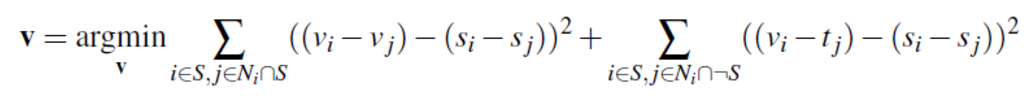
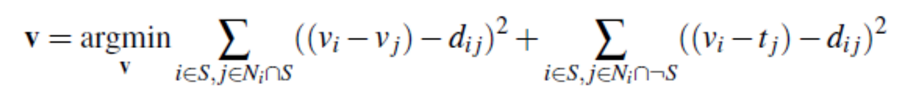
In other words, if we are given a matrix values representing the gradients between neighboring pixel intensities:

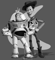
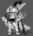
and a single pixel intensity value, we should be able to reconstruct the original image by expanding intensity values out from the given pixel, using the gradients. The first image below is an example original, the second, the reconstructed version.

I was able to reduce the execution time of this reconstruction significantly (from around 15 seconds to around 4 seconds) by building the sparse constraint matrices via vectorization.

Poisson Blending

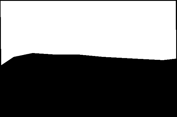
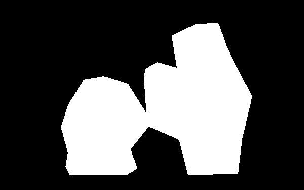
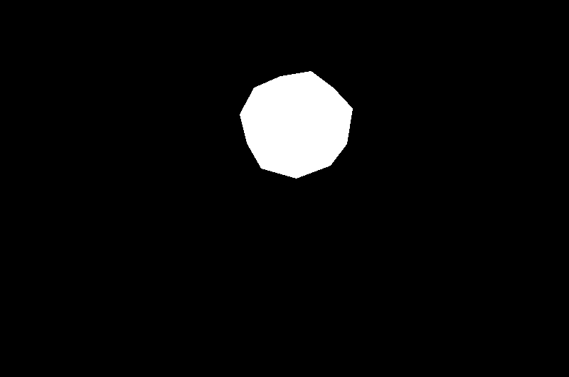
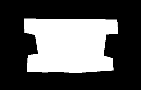
One way to blend in image into another is with Poisson blending. There are two images: a source image, and a target image in which we want to place the source image. We create a mask that selects the portion of the source we want to blend into the target. Then, we set up the following constraints:

Pixels in the target image that aren't in the masked area should be close to the intensity values in the target.
The gradients of pixels in the masked area should be constrained to have close to the gradients of those in the source image.

Here are some results of Poisson blending:

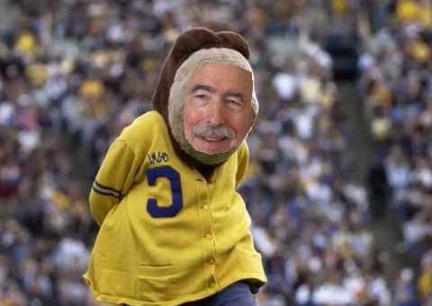
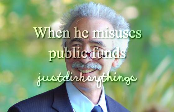
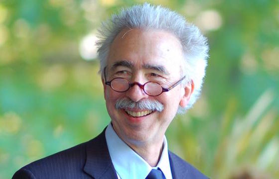
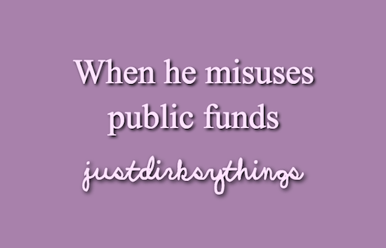
Dirski

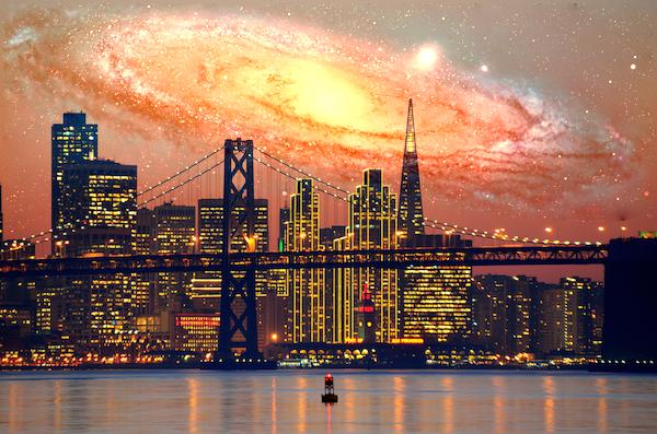
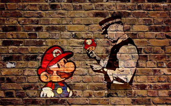
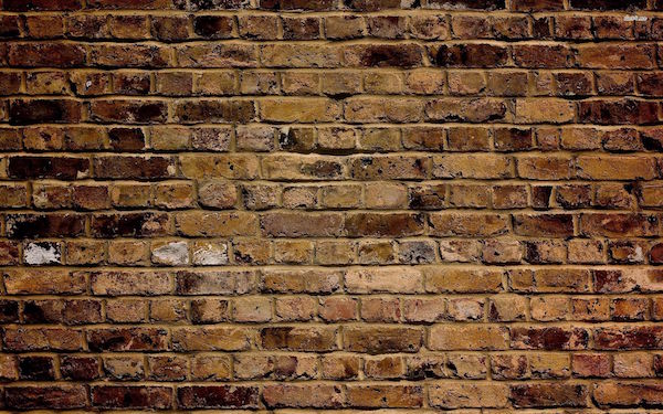
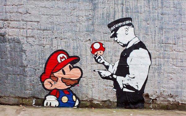
Mixed Gradients

Mixed gradients is just like Poisson blending, except we constrain the gradients of the pixels in the masked area to be the gradient of those in the source image OR target image: whichever has a larger magnitude. Note that this gradient choice is made on a per-gradient basis.

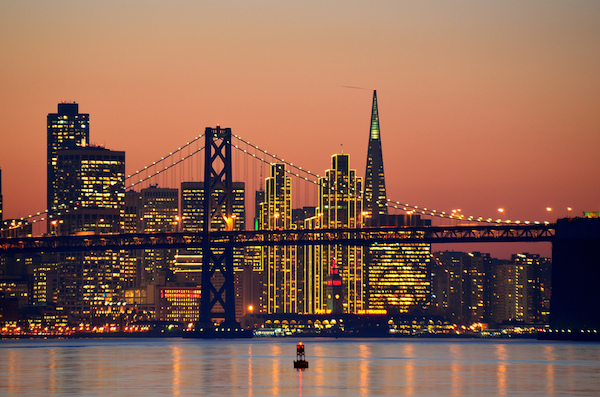
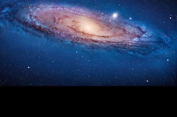
d_ij is the value of the gradient from the source or the target image with a larger magnitude

SF Skyline • Notice that the mixed gradients allow the tall buildings and the bridge to appear in front of the galaxy.

Banksy on Brick • The colors of the original piece are preserved, but toned to match the bricks. The brick texture also prevails because of its larger gradients.

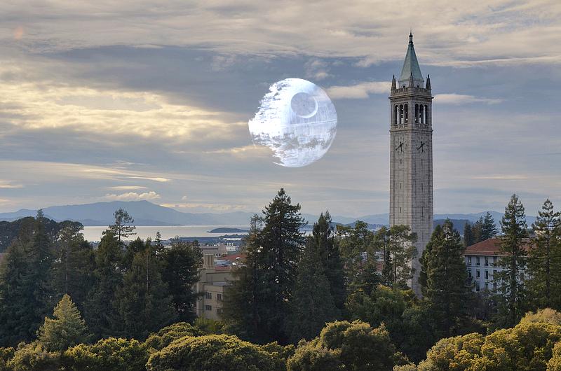
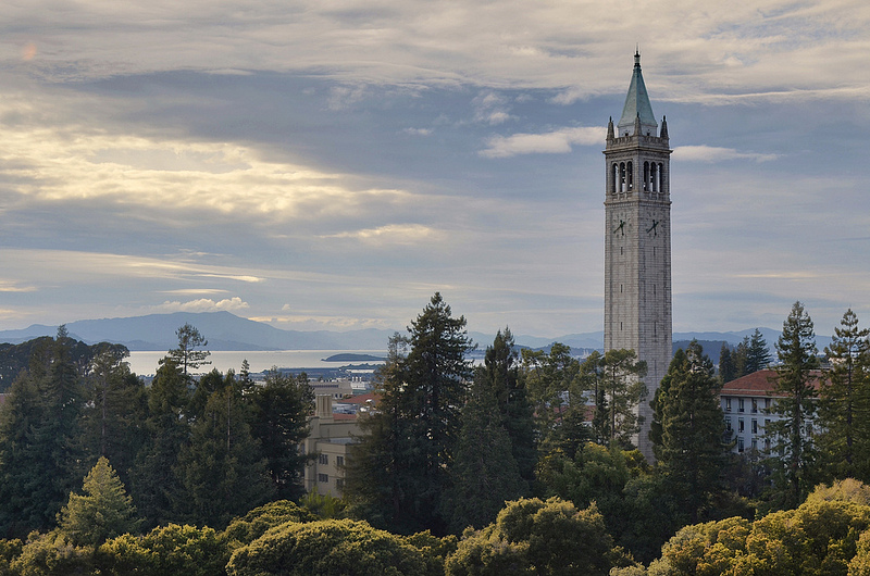
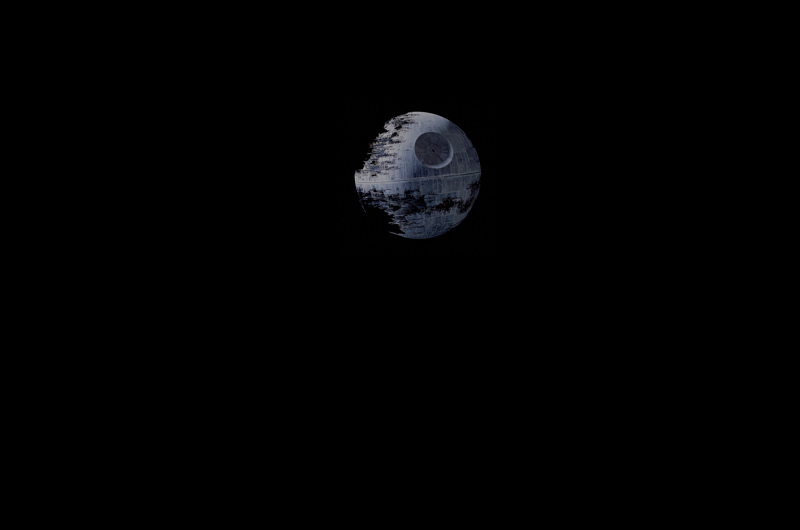
That's No Moon • The Death Star is faded to more match the brightness and color of the sky. Notice how the clouds float in front of the Death Star. Without mixed gradients, the clouds would simply fade out and become blurry when they got to the masked region.

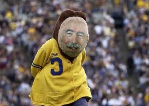
Just Dirksy Things • Writing can be applied over images with mixed gradients. Notice how the pink background is completely disregarded because of its virtually zero gradient, while the words stand out due to the high gradient between the pink and letters.

Vs. Laplacian Pyramid Blending

Laplacian blending is another cool way to blend images. Here’s a case when Poisson blending is clearly the way to go:

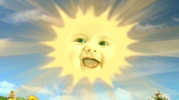
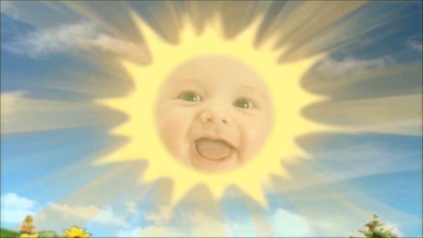
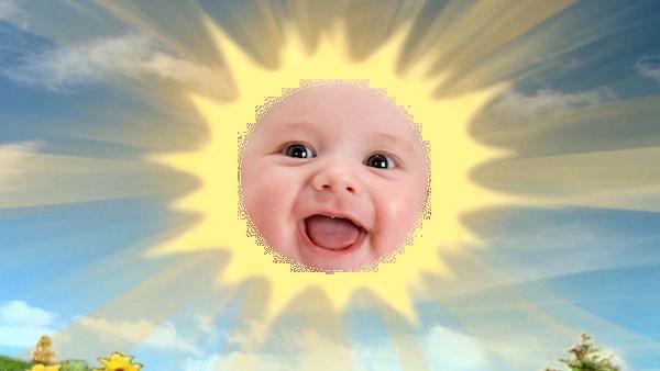
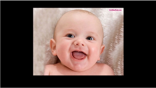
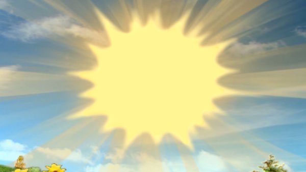
Poisson blending was much better than Laplacian blending in this case. This is because Poisson blending was able to make the overall color palette of the baby match that of the sun, which is the intended effect. Laplacian blending can’t and doesn’t achieve that effect. Laplacian blending can be better when Poisson blending would cause an unwanted color shift.

◼