Cloth Simulation

Overview

How would you approach making a realistic animation of a waving flag? Would you study a video of a real flag and draw each frame? That would take a long time. Would you develop a mathematical model that describes how flag surfaces move? It may be difficult to bridge the last gap between that ‘fake’ look and realism.

A good way to approach it is to describe the cloth’s physical properties, the world, and physics the best we can, and “press play”. That is to say, create a simulation of the flag. The problem is open ended: How do we model the cloth? What information about the environment is important? I explored these ideas while creating a cloth simulation.

Masses and Springs

A good model for a cloth is a bunch of small masses and springs. A square cloth is broken up into a grid of points, instead of some continuous representation. This way, we can apply forces to a finite number of objects. Further, this makes modeling a cloth’s elastic properties easier. We can connect the point mass objects with a system of tiny springs that keep the cloth from contorting in an unnatural way. Springs act as a constraint on distance: applying a force to push away objects that are too close, or applying tension between objects that are too far.

I incorporated three types of springs into the cloth model: structural, shearing, and bending.

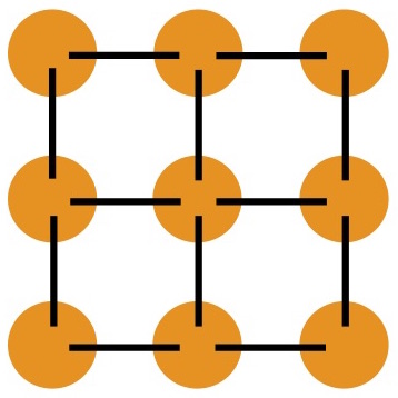
Structural springs exist between each mass in a row and column fashion. They make sure the overall topology of the cloth remains consistent. They also prevent neighboring masses from being pulled apart or pushed together.

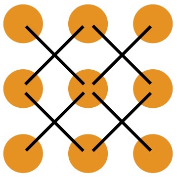
Shearing springs reach between diagonal masses. These prevent the entire grid from collapsing to one side, like parallelogram collapsing onto its side.

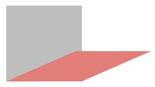
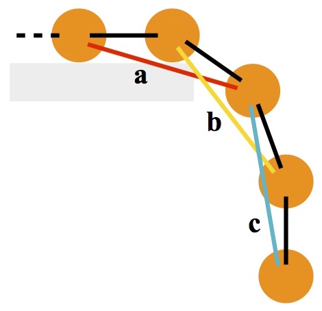
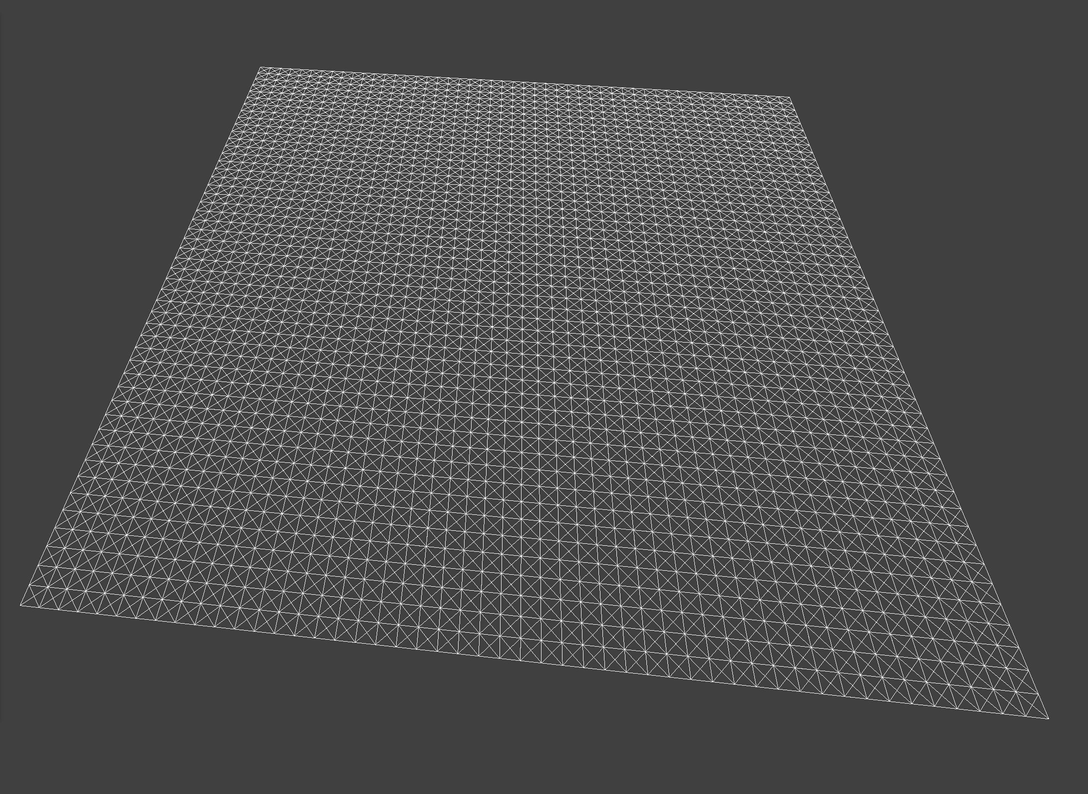
Lastly, bending springs span two masses, and prevent the cloth from creasing perfectly in half like an infinitely thin piece of paper, which would be unrealistic. In the following image, the effect of bending constraints can be seen.

The following image shows the springs as white lines in an example cloth. A shaded version of this cloth will be used in the simulations.

Simulation via numerical integration

I implemented verlet integration to simulate the cloth. Verlet integration is a method of updating the point mass positions based on the forces acting on them at the given instant. It scales with the speed of the simulation, and can be damped. At each step of the simulation, verlet integration looks at every point mass in the system, aggregates the forces that are acting on it and moves the point mass to a new position based on these forces. In this case, the important forces are due to gravity and springs.

Default parameters

Here is what a 4 corners pinned cloth looks like with the default parameters. You can reset the simulation by pressing the "reset" button.

reset

Varying spring constant

A spring’s strength is determined by its spring constant, denoted as ks. This number determines how strongly the strings pull on the masses in the cloth. Below, I simulate two cloths: one with a low ks, and one with a high ks. The normal ks is 5000.

reset both

In the low ks simulation (on the left), the cloth dips much further down than the high ks simulation (on the right). Before it comes to rest, waves in the cloth are also much more pronounced in the low ks simulation. The high ks simulation comes to rest before the low ks simulation.

Varying density

The density of the cloth changes the mass of each point that the cloth is comprised of. Changing the density of the cloth changes the degree to which it is affected by forces. Below, I simulate low and high density cloths. The default density is 15.

reset both

One thing to quickly notice is that the high density cloth behaves like the low ks cloth, and the low density cloth behaves like the high ks cloth. The only difference separating the changes in ks and density is that changes in ks affects the spring force contribution, while changes in density affect both spring and environmental force contributions.

Varying damping

Damping controls how quickly our simulation loses energy. It is implemented in the verlet integration step of the simulation. Below, we simulate a cloth with low damping and high damping. The default damping value is 0.2.

reset both

The low damping simulation takes a very long time to come to rest. Small changes ripple throughout the length of the cloth well after their inception. In the over-damped simulation, the opposite occurs: the cloth smoothly falls into a resting position, with virtually no waves propagating. Notice, however, that the over-damped simulation does not come to rest in the exactly the same way as the default simulation! (scroll back up to see the default simulation).

3: Handling collisions with other objects

To create a collision with a sphere, the following steps are taken:

1. If a point mass is inside a sphere object:
2. Bump it away from the sphere's origin to the surface.
3. Correct its distance from its last position by a little bit, influenced by some friction value of the sphere.

This algorithm allows the cloth to avoid being inside of another object. I implemented the algorithm and simulated a cloth falling over a sphere, varied across ks values.

Collision with a sphere

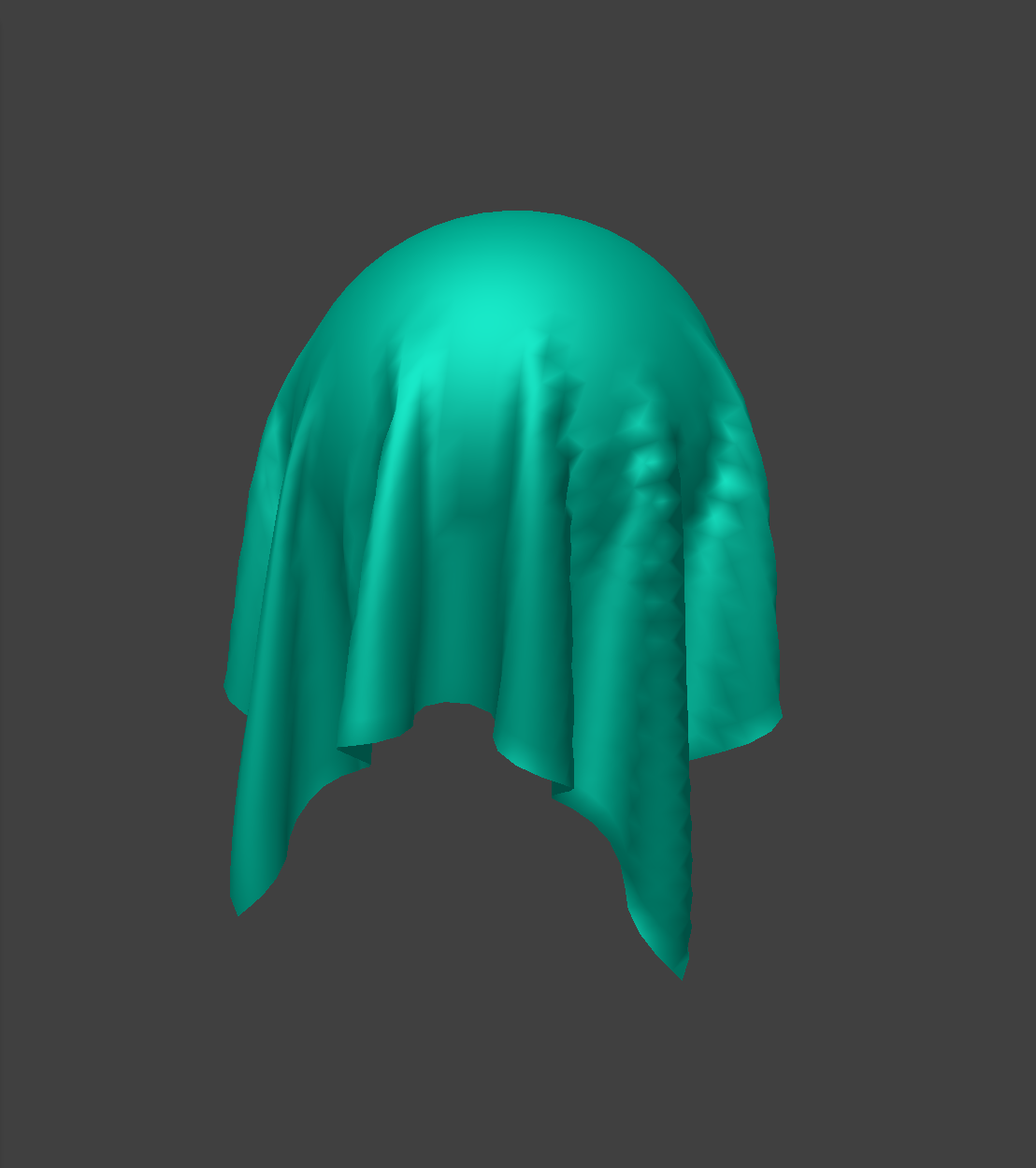
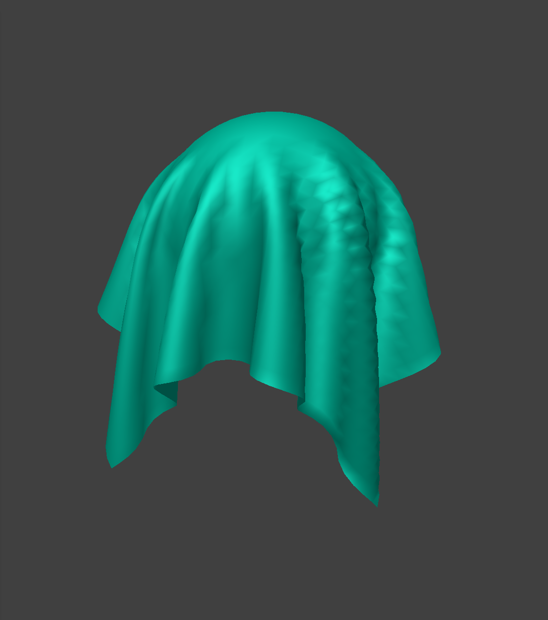
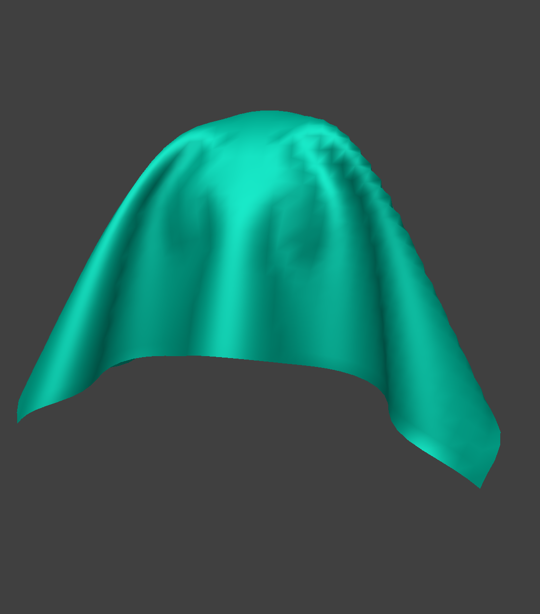
The first cloth looks like a very fine material, such as silk. The last cloth looks like a stiff material, such as felt. This is due to the varied spring constant values. For example, the material on the right (felt-like) has a high spring constant, so the cloth is more resistant to shearing and bending.

Collision with a plane

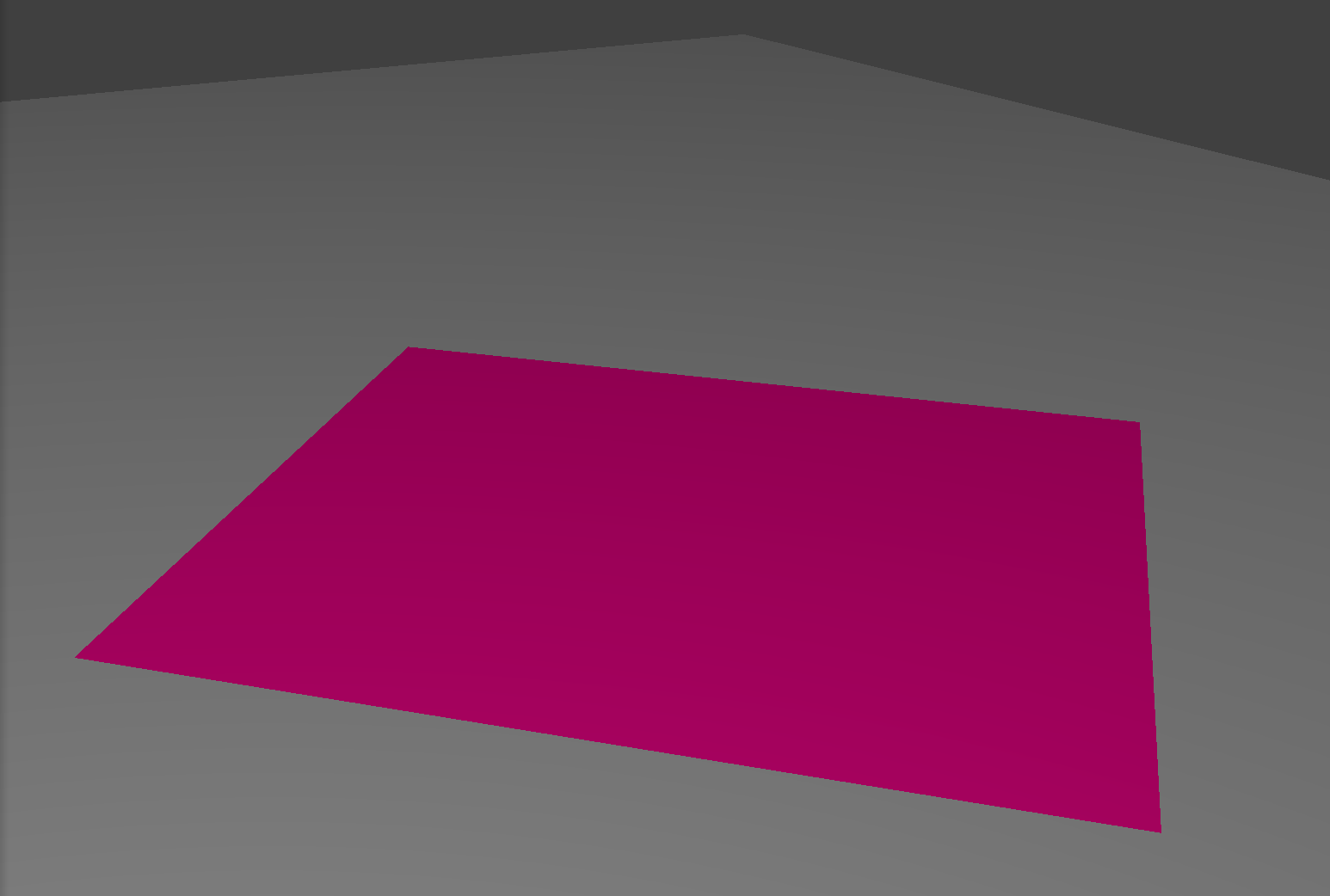
A similar process is implemented to detect collisions with planes. The test to see whether a collision occurs involves testing whether a point mass moves to the other side of a plane on a given simulation step. Below is the result of a cloth falling onto a plane and colliding with it.

4: Handling self-collisions

To handle self-collisions, point masses in the cloth need to be tested against each other to see if their positions are smaller than double the thickness of the cloth. The naive solution would test every point against every other point, and this would be O(n^2). We can do better.

To get better than quadratic in the number of point masses, we can test point masses only against their spatial neighbors. To do this, we first place all point masses into buckets based on their location in 3D space. This is called Spatial Hashing. We treat 3D space as a grid of boxes and iterate over every point mass, determining which box each of them lies in. Then, we go through all boxes, and test the all of the points in each against each other. This way, we only test a point against those in the same box, instead of against ALL other points. This saves a lot of time, and for a typical cloth simulation, will be O(n).

Spatial hashing involves the ability to uniquely identify each box that we've divided the 3D space with. The way I chose to do this is as follows:

1. Figure out the coordinates of the position in question in the new "box-space".
2. Multiple each component of the new basis position by a large prime and XOR them together.

This is a simple but somewhat common hashing scheme.

Below, I've simulated a vertical falling cloth that collides with itself.

reset

As we can see, the cloth folds over itself instead of moving through itself. There are only a couple of frames in which the cloth intersects with itself, and these situations are infrequent. The reason this happens is because of the spatial hashing scheme: Imagine two points that are very close to each other, but fall into separate 3D boxes because their positions are near those boxes' borders. They would not get tested against each other for closeness! I revisit this problem later in part 5.

Varying density

Below, I vary the density of the cloth, then simulate the self-collision situation.

reset both

With low density, the spring forces keep the cloth very rigid, and it folds neatly. With high density, the cloth folds messily as the point masses quickly succumb to an increased ratio of environmental to spring forces.

Varying spring constant ks

Below, I vary the spring constant ks, then simulate the self-collision situation again.

reset both

Similarly to the 4 corners pinned cloth earlier, it is apparent that density and ks have something of an inverse relationship in how they affect the cloth. This time, the low spring constant allows the cloth on the left to fold over on itself more easily, while the high spring constant in the cloth on the right keeps it more rigid and structured.

5.1: Wind

Wind is a spatially varying environmental force. I had fun imagining the components of an overall force due to wind. I also got to have fun using the vector field functionality of Grapher, an OSX utility, to help me visualize my wind construction.

I imagined that wind not only varies through space, but also time. To implement this properly, I kept track of the total amount of time since the simulation began. I used this to parameterize my wind force.

I built the wind up in three steps:

1. Varying the force over the z axis w/ respect to time
2. Varying the force over the y axis w/ respect to time
3. Adding a slight oscillating perturbation in the x axis w/ respect to time

Below, I show the vector fields animated over time as I add each component above.

5.2: Accurate self-collisions

Remember the problem addressed at the end of section 4? In that two points may lie very close to one another but lie in separate 3D boxes? One way we can fix this is to not just search the bucket the point in question lies in while checking for closeness, but instead, check in all the neighboring buckets. This way, we sacrifice some speed for correctness. I'm not sure what this scheme is called, but I've nicknamed it Uniform Spatial Hashing.

To do this, I needed to improve the hashing scheme for a box, because I needed a way to retrieve neighbor boxes once they've been hashed. To solve this, I moved from using doubles to identify boxes to using 3D tuples to identify boxes. I had to write a 3D tuple-compatible unordered map in order to do this, but luckily I was able to reuse the idea behind hashing scheme I wrote for the doubles, with XOR.

Now that a box's neighbors were identifiable, I just made sure I included all of the neighboring boxes in the search space when checking for closeness of point masses.

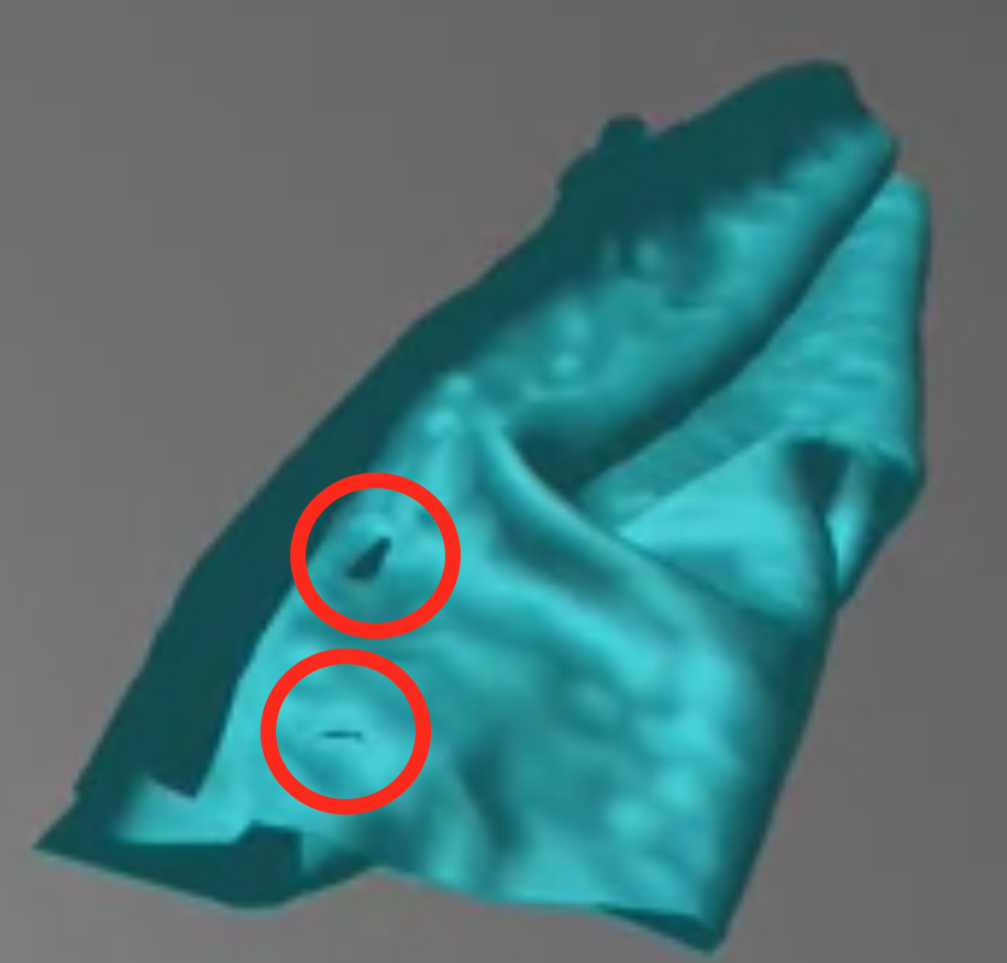
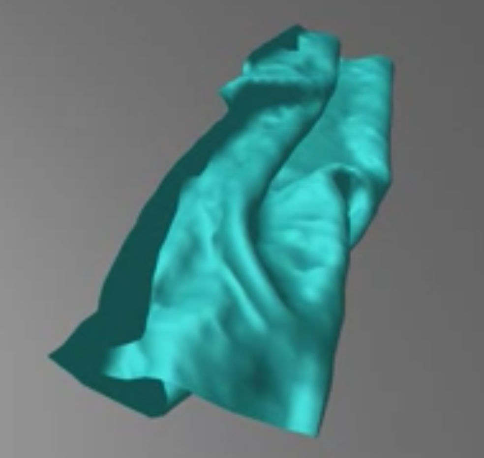
Below, I simulate self-collision examples before and after the accuracy-boosting spatial hashing system.

reset both

Did you catch the improvement? I've captured a screengrab of the cloth in similar positions in each simulation so you can see the difference. The results are below:

That's it for my experiments with cloth simulation. Thanks for reading! ◼