How to Get 97% on MNIST with KNN
Get the data
This Kaggle competition is the source of my training data and test data. I also used it to calculate the final test score.
Numpy’s genfromtxt function is an easy way to get the .csv data into a matrix:
import numpy as np
X = np.genfromtxt('data/train.csv', delimiter=',',
                  skip_header=1).astype(np.dtype('uint8'))
However, it’s slow, especially if you’ll be rerunning your program and reloading the data a lot. I recommend serializing the numpy matrix with the pickle module after the first load, and loading the saved pickle object on all subsequent runs of your program.
import pickle
with open('data/train_points.p', 'wb') as f:
    pickle.dump(X, f)
...
with open('data/train_points.p', 'rb') as f:
    X = pickle.load(f)
Write KNN
KNN is fun to me because it trains in order 0 (zero) time. Here’s the setup for the actual implementation:
class KNN:
    def __init__(self, data, labels, k):
        self.data = data
        self.labels = labels
        self.k = k
Predictions are where we start worrying about time. We’ll worry about that later. For now, let’s implement our own vanilla K-nearest-neighbors classifier. In the predict step, KNN needs to take a test point and find the closest sample to it in our training set. We’ll use the euclidian metric to assign distances between points, for ease.
Take the difference between all of the data and the incoming sample point at once with numpy’s element-wise subtraction: differences = self.data - sample. Then, to complete the distance calculation, take a row-wise inner product between differences and itself. Numpy’s einsum provides a fast execution. Lastly, get the k smallest distances and their corresponding label values. Here’s the final implementation:
from scipy.stats import mode
class KNN:
  def predict(self, sample):
      differences = (self.data - sample)
      distances = np.einsum('ij, ij->i', differences, differences)
      nearest = self.labels[np.argsort(distances)[:self.k]]
      return mode(nearest)[0][0]
Improve with PCA
Our KNN currently considers all 784 features for each image when making its decisions. What if it doesn’t need that many? It’s possible that a lot of those features don’t really affect our predictions that much. Or worse, KNN could be considering feature anomalies that are unique to our training data, resulting in overfitting. One way to deal with this is by removing features that aren’t contributing much. Taking this concept further, better features, made up of linear combinations of the original features could be discovered. The original features are referred to as “axis aligned”, because our data is plotted against these feature axes. By finding better non-axis-aligned features, a new coordinate system for our data can be created composed of axes that run in more important directions (that is, the training data has higher variance along these axes). For a visual explanation, consider the following picture of a group of data:
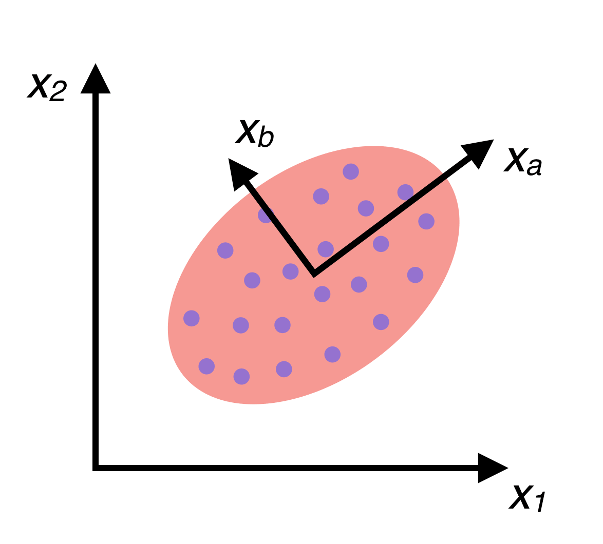
If the data is fit to a Gaussian distribution, one can see that there are two eigenvectors which, if used as a basis when plotting the data, could provide a much higher variance among the data than our \(x_1\) and \(x_2\) axes. In other words, these two directions \(x_a\) and \(x_b\) tell us more about the data than \(x_1\) and \(x_2\). Finding \(x_a\) and \(x_b\) and plotting our data in a new coordinate system based on these axes is called Principal Components Analysis (PCA).
Continuing from this idea of finding the eigenvectors that best describe our data, let’s talk math. Let \(X\) be a design matrix, \(nxd\). If we assume \(X\) is centered, then its covariance matrix is \(X^TX/(n-1)\), which can be decomposed as \(V L V^T\), where \(L\) is a diagonal matrix composed of decreasing eigenvalues of the covariance matrix. \(V\) is made of their corresponding eigenvectors. The first \(k\) eigenvectors are the first \(k\) most important directions when it comes to our data. If we take \(XV\), we get the projection of \(X\) onto \(V\), placing the data in \(X\) into a basis that maximizes the variance of that data. The new and improved data is now composed of better, linearly uncorrelated variables that we call principal components.
Now, computing \(X^TX\) is not cheap: it takes \(O(nd^2)\) time. Luckily, to the rescue comes the Singular Value Decomposition (SVD). SVD can break our \(nxd\) design matrix into \(X = UDV^T\), where \(U\) is composed of vertical left singular vectors of \(X\), which are all orthogonal to each other. Similarly, the rows of \(V\) are the right singular vectors of \(X\). \(D\) is diagonal, and its entries are the nonnegative singular values of \(X\). At any rate, observe that the covariance matrix of \(X\) is estimated by \(X^TX/(n-1)\) \(=VDU^TUDV^T/(n-1)\) \(=VD^2V^T/(n-1)\). The principal components are given by \(XV = UDV^TV = UD\). Taking the first \(k\) columns of \(U\) and the first \(k\) entries of \(S\) gives us \(U_kD_k\), the estimation of \(XV\) using only the first \(k\) principal components. In the end, we can find the \(k\) greatest singular values and their corresponding vectors in \(O(ndk)\) time. If \(k\) is chosen to be something like 40, then that’s a big time saving from 784 original dimensions.
I used numpy’s linalg package to solve the SVD of the design matrix. Here’s my function for using the SVD to find the PCA of the data (don’t forget to center the data).
def svd_pca(data, k):
    """Reduce DATA using its K principal components."""
    data = data.astype("float64")
    data -= np.mean(data, axis=0)
    U, S, V = np.linalg.svd(data, full_matrices=False)
    return U[:,:k].dot(np.diag(S)[:k,:k])
Reducing the dimensionality of the MNIST data with PCA before running KNN can save both time and accuracy. Lower dimensions means less calculations and potentially less overfitting.
Cross Validation
Now the data can be preprocessed from an original dimension of 784 to some \(k\) « 784. There are two last questions: How many nearest-neighbors should we use in KNN? And how many dimensions should we reduce our data to through PCA?
When in doubt, cross validate. I set up a two dimensional cross validation test, and plotted the results:
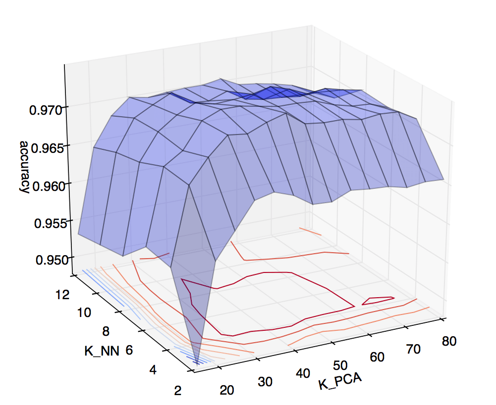
On the vertical axis is accuracy obtained via cross validation. On the horizontal axes are \(k\) for KNN, ranging from 2 to 12, and \(k\) for PCA, ranging from 5 to 80. The heat map on the lower plane helps illustrate that the best accuracies were achieved around \(k_{NN} = 6\), \(k_{PCA} = 45\). So, these are the values I used to predict on the Kaggle test set. Kaggle scored the submission at just over 97%. Not bad for around 12 lines of code (and numpy’s SVD solver)! ◼